
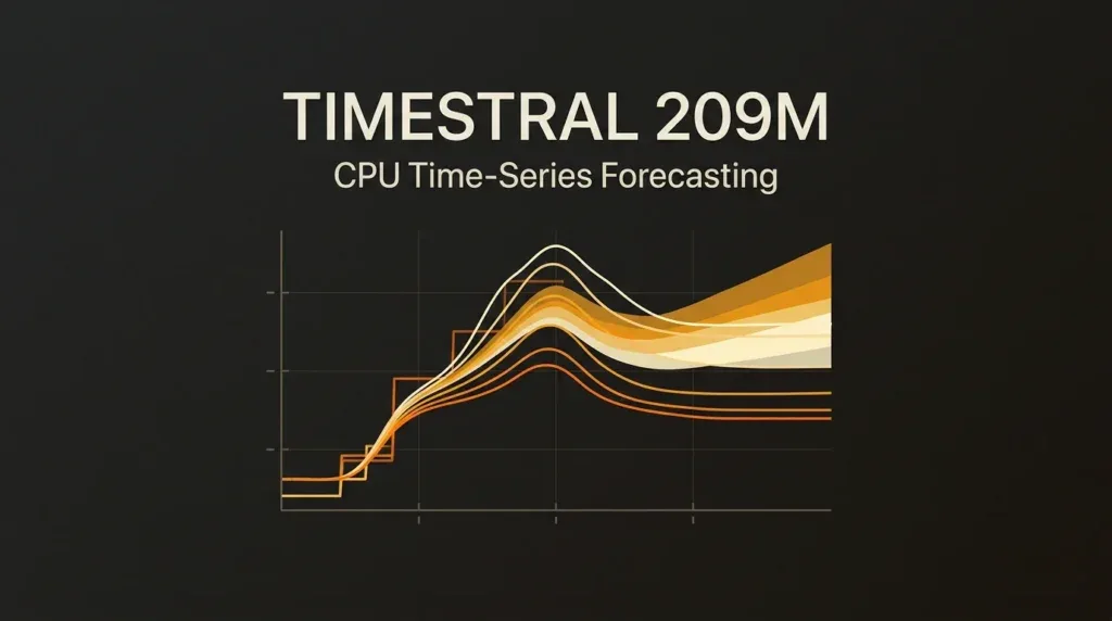

Mistral Timestral deploys a 209-million-parameter time-series foundation model capable of generating 21 probabilistic quantiles across 1,024 forecast steps from a 32,768-step context in 140 milliseconds on standard 8-thread server CPUs. Operating entirely within an 837-megabyte memory footprint in FP32, it replaces GPU-bound forecasting clusters with lightweight, deterministic local CPU execution.
For two years, enterprise machine learning infrastructure has been governed by an expensive assumption: deploying foundation models requires reserving multi-GPU server clusters, paying exorbitant cloud rental fees, and engineering complex tensor-parallel serving stacks. While generative text architectures have scaled into hundreds of billions of parameters, industrial time-series forecasting has operated under entirely different physical constraints. Production telemetry—such as factory sensor streams, data center power loads, server cluster memory metrics, and financial exchange order books—demands millisecond-level responsiveness, deterministic execution, and low inference costs.
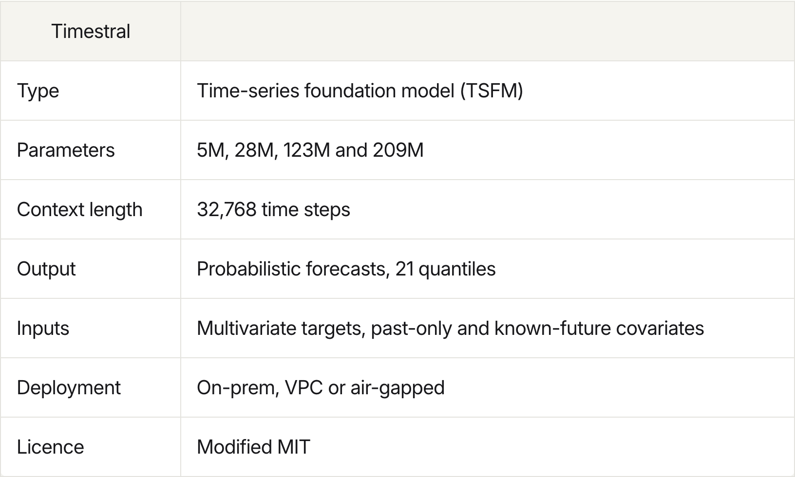
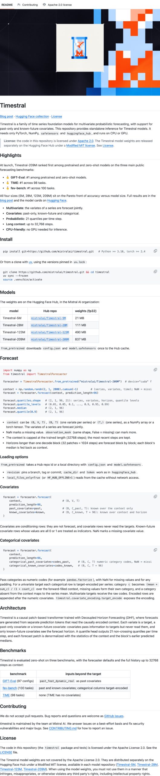
Mistral AI entered this domain with Timestral, a family of zero-shot time-series foundation models spanning 5 million, 28 million, 123 million, and 209 million parameters. Rather than requiring specialized accelerator clusters, Timestral is architected to run directly on standard x86 and ARM server processors. The largest 209M parameter variant occupies a mere 837 MB of system memory in single-precision floating point (FP32), while the entry-level 5M parameter variant requires just 21 MB, comfortably fitting inside the level-3 (L3) cache of modern AMD EPYC and Intel Xeon processors.
This architectural shift mirrors the hardware bifurcation we analyzed across local edge models: while large language models struggle with memory bandwidth ceilings—a phenomenon detailed in our evaluation of Nemotron 3.5 Bolt VRAM requirements and the unified memory limits explored on Liquid AI LFM2.5-24B on Apple M5 Max—specialized numerical sequence transformers can operate entirely inside host CPU memory without PCIe bus transfer latency.
Yet beneath Mistral’s marketing claims of zero-shot Pareto optimality across industrial benchmarks lies a severe operational reality. Time-series data does not behave like natural language. When production engineers feed messy real-world covariates into Timestral without understanding its underlying patch projection mechanics, the model’s forecasting reliability collapses.
The Covariate Sensitivity Trap
The fundamental limitation of transferring transformer architectures from text to time series lies in the absence of a universal semantic vocabulary. In natural language, tokens possess intrinsic semantic relationships embedded during pretraining; words like “holiday” or “downtime” carry rich contextual priors. In numerical time series, however, covariates are raw scalar floating-point arrays.
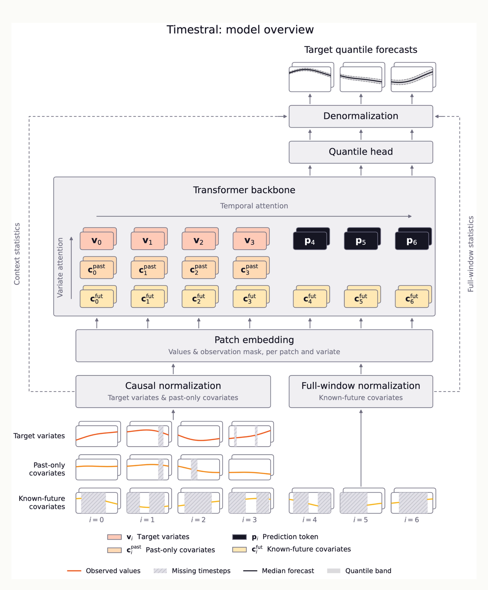
Timestral processes historical sequences by grouping continuous time steps into fixed patches of 32 observations each. When exogenous covariates—such as promotional flags, ambient temperature, electricity spot prices, or calendar indicators—are fed alongside target time series, the model projects both the values and their corresponding observation masks into a unified latent dimension.
This introduces what systems engineers call the Covariate Sensitivity Trap. In standard tabular machine learning pipelines utilizing gradient-boosted decision trees (LightGBM, XGBoost, or CatBoost), missing values are routinely filled with zero or imputed using forward-fill heuristics. In Timestral, zero-filling missing covariate observations creates catastrophic distribution shifts. Because zero is a valid physical measurement (representing 0 Watts of power consumption, 0 RPM motor speed, or a baseline calendar index), the patch linear projection treats an imputed zero as a continuous physical measurement.
To maintain calibration across its 21 output quantiles, Timestral requires missing values to be explicitly formatted as NaN (numpy.nan). When the patch embedding encounters an explicit NaN, it sets the corresponding observation mask bit to zero, preventing the unobserved step from corrupting the continuous causal normalization layer. If an engineer accidentally zero-fills an offline telemetry sensor during a data ingestion outage, Timestral treats the zero as a massive real-world drop, causing the 1,024-step quantile forecast fan-out to explode in variance.
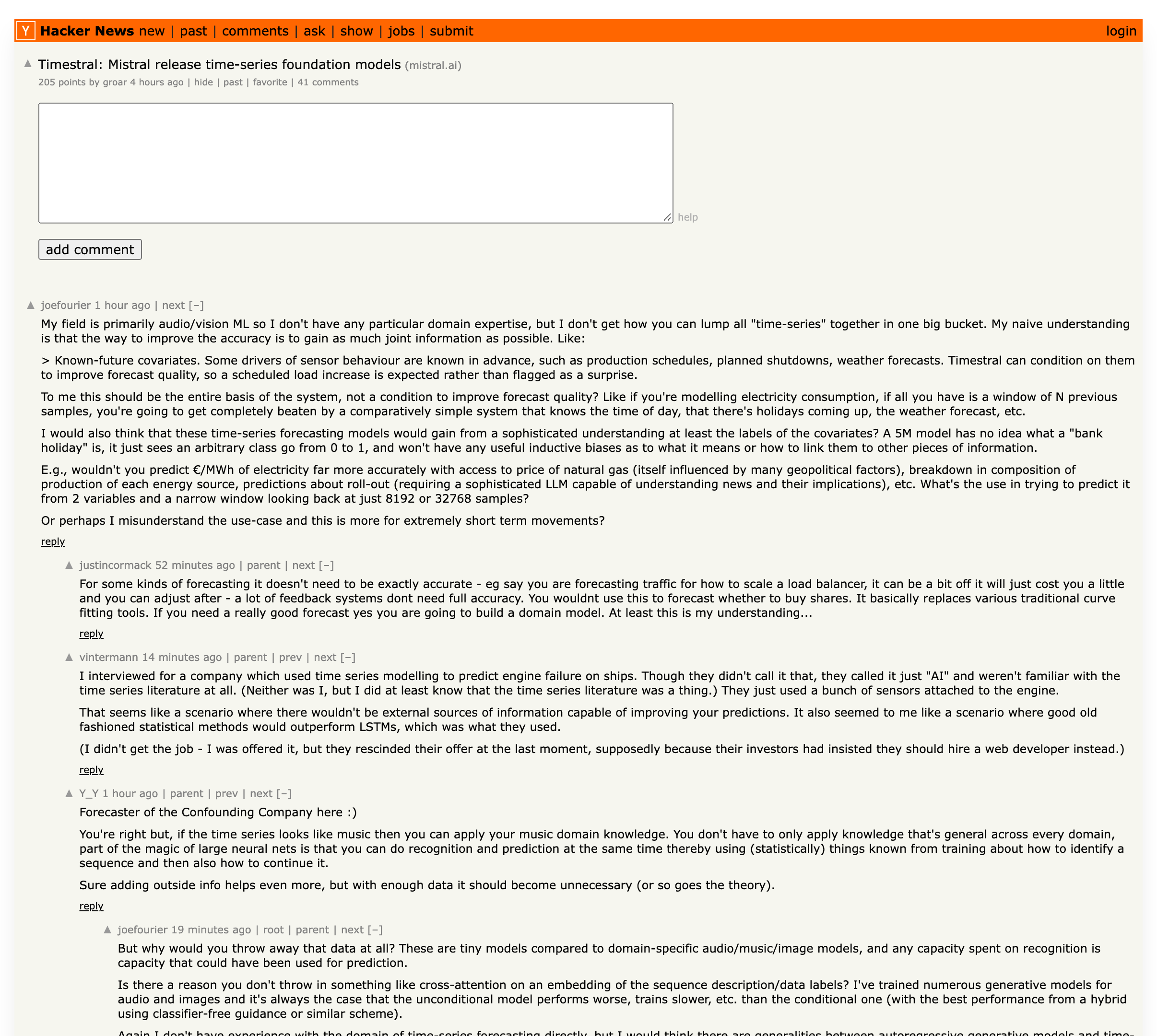
Beyond missing data mechanics, smaller foundation models suffer from severe semantic blindness. As noted by forecasting engineers discussing Timestral’s release on Hacker News, a 5-million or 28-million parameter model possesses zero internal world model. When provided with an integer covariate indicating a national bank holiday, the model does not “understand” that commercial retail traffic will drop while residential streaming bandwidth will spike. It treats the indicator as an arbitrary binary state transition from 0 to 1. In industrial settings where exogenous calendar anomalies dictate outcomes, a simple gradient-boosted tree with domain-engineered holiday features consistently outperforms a zero-shot neural foundation model that lacks external semantic context.
Relying on remote hosted endpoints also introduces severe operational friction. During European business hours, developers utilizing Mistral’s preview API reported severe latency jitter and connection timeouts, echoing the hosted infrastructure bottlenecks documented in our teardown of DeepSeek Flash 1017 API pricing and latency. For systems engineers responsible for automated industrial dispatch, relying on remote cloud APIs for millisecond-level telemetry forecasting is an unacceptable architectural risk. The only robust deployment topology is local CPU execution on owned hardware.
Decoupled Horizon Architecture and CPU Memory Scaling
To understand how Timestral achieves 140-millisecond inference on commodity CPUs without GPU acceleration, one must examine its Decoupled Horizon Forecasting (DHF) architecture.
Classical autoregressive time-series transformers generate predictions one step at a time, feeding each generated prediction back into the context buffer. For a 1,024-step forecast horizon, this requires 1,024 sequential forward passes, creating severe latency bottlenecks. Timestral eliminates this through patch-based parallel generation and decoupled horizon tokens.
Historical context is accepted up to 32,768 time steps, which the model slices into 1,024 patches of length 32. In parallel, the forecast horizon of 1,024 steps is represented by 32 discrete prediction tokens (p1, p2, …, p32). These prediction tokens attend to the historical context representations through a 2D attention transformer backbone that computes attention across two distinct axes:
- Temporal Attention: Calculates dependencies across historical time patches along the sequence dimension.
- Variate Attention: Calculates cross-channel correlations across target series, past-only covariates (cpast), and known-future covariates (cfuture).
Because prediction tokens only read context tokens and do not allow context tokens to attend forward into the forecast window, Timestral generates all 1,024 future steps across all 21 quantiles in a single forward pass.
The model also separates normalization into two distinct pathways:
- Causal Normalization: Applied to target variates and past-only covariates, calculating running mean and variance strictly over historical context to prevent future leakage.
- Full-Window Normalization: Applied to known-future covariates (such as planned maintenance schedules, forecasted ambient temperatures, or scheduled pricing tariffs), normalizing across the entire combined context and forecast horizon.
When categorical covariates are present, Timestral requires continuous numerical projection prior to patch ingestion. Categorical features are converted using smoothed target encoding:
Smoothed Target Encoding for Categorical Covariates
Converts discrete categorical indicators (e.g. store IDs, product SKUs, regional tariffs) into continuous scalar channels required by Timestral’s 2D spatio-temporal patch embedding layer prior to cross-channel variate attention.
Architectural Imperative: Unlike natural language LLMs that assign high-dimensional discrete embedding vectors to arbitrary tokens, time-series foundation models pass all inputs through continuous numerical patch projections. Passing raw categorical integers (such as Store ID 104 vs. 105) corrupts 2D attention matrices with artificial ordinal relationships. Smoothed target encoding maps discrete metadata onto an empirical continuous scale without inflating the model’s variate channel dimension or causing overfitting on low-frequency classes.
On physical hardware, this architecture translates to remarkably modest memory requirements:
Whereas even small quantized large language models demand between 6 GB and 16 GB of system RAM—as explored in our deployment guide on How to Run Bonsai 2 9B GGUF—Timestral-209M fits easily into entry-level single-board computers, edge IoT gateways, or low-cost cloud instances with only 1 GB of allocated RAM.
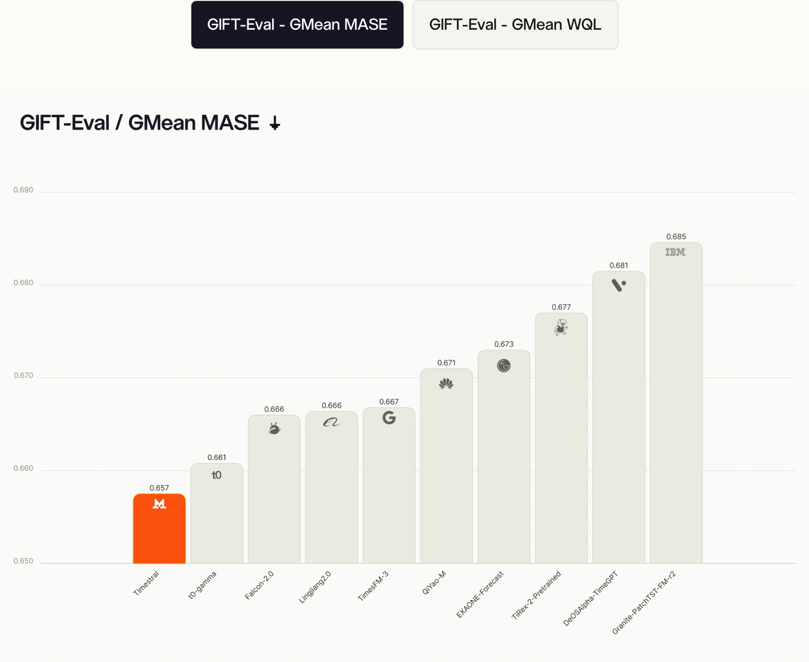
On verified zero-shot benchmarks, Timestral establishes competitive numbers. On the standardized GIFT-Eval suite, evaluated using the Geometric Mean Mean Absolute Scaled Error (GMean MASE, where lower scores represent superior accuracy), Timestral-209M scores 0.657, leading the foundation model class ahead of open competitors including t0-gamma (0.661), Falcon-2.0 (0.666), and Google’s TimesFM-3 (0.667).
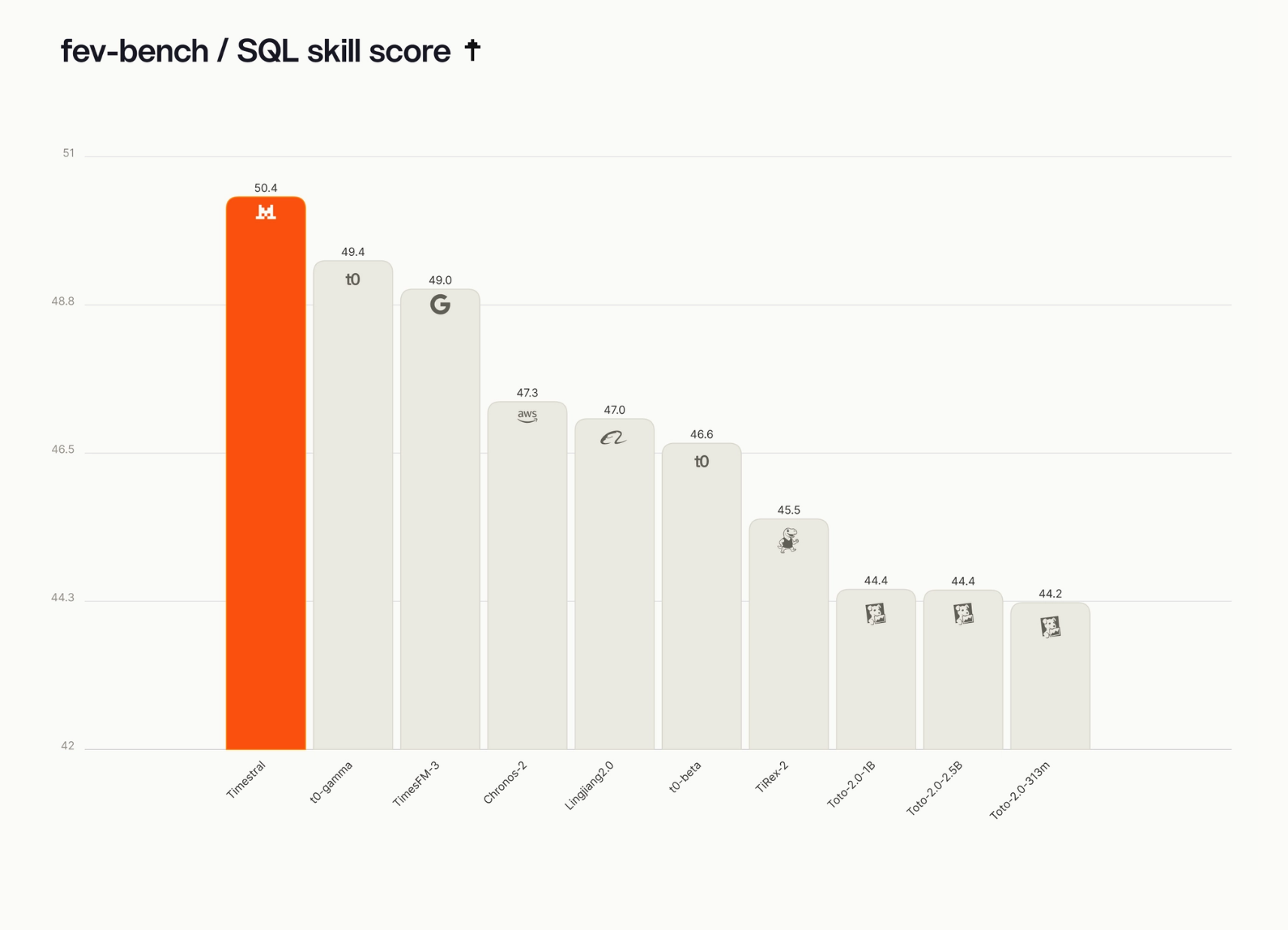
Similarly, on fev-bench across 100 industrial forecasting tasks evaluated by SQL skill score (where higher scores indicate superior accuracy), Timestral-209M achieves 50.4, outperforming Google’s TimesFM-3 (49.0) and Amazon’s Chronos-2 (47.3). However, open rival t0-gamma from The Forecasting Company trails by just 1.0 point at 49.4, achieving a 42% head-to-head win rate across the same evaluation distribution.
Foundation Model Accuracy: GIFT-Eval vs. fev-bench
Comparing Mistral Timestral-209M against major time-series foundation models across academic zero-shot error (GIFT-Eval) and real-world SQL forecasting skill (fev-bench).
t0-gamma stays within 1.0 point on enterprise SQL workloads, capturing a 42% head-to-head win rate on tasks dominated by external covariate interactions. When exogenous features are poorly aligned, foundation model depth cannot compensate for semantic blindness.Local CPU Deployment and Standalone Inference
Running Timestral on local hardware requires no proprietary CUDA drivers, ROCm libraries, or specialized container runtimes. The official inference implementation relies on standard NumPy and PyTorch execution.
To demonstrate how the model handles exogenous covariates and missing value masks, the following production script executes standalone CPU inference with explicit NaN handling on standard server hardware:
import numpy as np
import torch
from timestral import TimestralForecaster

# Initialize CPU execution device
device = "cpu"
torch.set_num_threads(8)

# Load model weights from local disk or cache (837 MB for 209M variant)
forecaster = TimestralForecaster.from_pretrained(
    "mistralai/Timestral-209M",
    device=device,
    torch_dtype=torch.float32,
)

# Synthetic industrial telemetry: 1,024 historical steps across 1 target and 2 covariates
context_length = 1024
forecast_horizon = 128

# Target: Power consumption (MW) with simulated missing sensor reading
target_history = np.sin(np.linspace(0, 50, context_length)) * 100.0 + 250.0
# Introduce a 16-step sensor dropout: MUST be np.nan, NEVER 0.0
target_history[400:416] = np.nan

# Past-only covariate: Ambient factory temperature (Celsius)
temp_past = np.cos(np.linspace(0, 25, context_length)) * 15.0 + 20.0

# Known-future covariate: Scheduled machinery operations (binary operational flag)
# Total length must span context_length + forecast_horizon
machine_schedule = np.zeros(context_length + forecast_horizon, dtype=np.float32)
machine_schedule[context_length : context_length + 64] = 1.0  # Scheduled run

# Format inputs into shape (Series, Variates, Time) as NumPy arrays
context = target_history.reshape(1, 1, context_length)
past_covariates = temp_past.reshape(1, 1, context_length)
known_covariates = machine_schedule.reshape(1, 1, context_length + forecast_horizon)

# Execute deterministic CPU forward pass
forecast = forecaster.forecast(
    context=context,
    past_covariates=past_covariates,
    known_covariates=known_covariates,
    prediction_length=forecast_horizon,
)

# Output shape: [batch_size, variates, forecast_horizon, 21_quantiles]
forecast_quantiles = forecast.quantiles.squeeze(0).squeeze(0)

# Extract critical operational quantiles across the horizon
q10 = forecast_quantiles[:, 2]   # 10th percentile (conservative lower bound)
q50 = forecast_quantiles[:, 10]  # 50th percentile (median forecast)
q90 = forecast_quantiles[:, 18]  # 90th percentile (risk-adjusted peak)

print(f"Inference complete: Generated {forecast_horizon} steps across 21 quantiles.")
print(f"Step 0 median forecast: {q50[0]:.2f} MW (90% range: {q10[0]:.2f} - {q90[0]:.2f})")
print(f"Step 63 median forecast: {q50[63]:.2f} MW (90% range: {q10[63]:.2f} - {q90[63]:.2f})")Memory Footprint: Timestral-209M vs. General LLM Architectures
How foundation time-series architectures circumvent the memory-bandwidth bottleneck that prevents standard generative LLMs from achieving deterministic real-time inference on edge and commodity CPUs.
Fits completely inside entry-level 1 GB VPS RAM. 140 ms CPU latency on 8 standard server threads allows 7 complete 1,024-step forecast cycles every second.
Requires 8 GB+ host memory once context buffers and KV caches expand. Autoregressive token decoding is severely constrained by DDR4/DDR5 system memory bandwidth.
Mandates dedicated hardware accelerators (e.g. RTX 4090 or A10G). Impossible to deploy on distributed IoT edges, air-gapped SCADA relays, or budget VPS tiers.
When integrating low-latency time-series models into enterprise data architectures, telemetry ingestion speed and index memory are often the real system bottlenecks. Pairing CPU-bound inference models with efficient database architectures—such as the memory compression techniques highlighted in our analysis of Timescale PRISM 100M vector storage on Postgres—ensures that retrieving 32,768 steps of historical context does not bottleneck the 140-millisecond inference execution.
The 1,024-Step Horizon Wall and Enterprise Licensing Friction
While Timestral’s single-pass generation of 1,024 steps is impressive on benchmarks, extending predictions beyond 1,024 steps exposes an architectural weakness: autoregressive error accumulation.
Because Decoupled Horizon Forecasting is capped at 32 prediction patches (1,024 time steps), generating a 2,048-step or 4,096-step forecast requires rolling autoregression. The engineer must take the median prediction (q50) of the first 1,024-step block, concatenate it to the historical context buffer, and execute a second forward pass.
In volatile industrial time series, point errors introduced in the synthetic median forecast feed directly into the causal normalization layer of the next block. By step 1,500, this feedback loop causes the outer quantiles (the 1st and 99th percentiles) to flare out into non-informative bounds. For forecasting horizons exceeding 1,024 steps, classical state-space models and structural seasonal models often preserve tighter calibration than multi-patch neural foundation models.
The second major enterprise friction point is intellectual property licensing. Mistral AI released Timestral under a dual-license structure:
- Code Repository: Apache 2.0 license, permitting commercial modification and integration of the Python harness.
- Model Weights: Governed by the Mistral Research License, strictly prohibiting commercial deployment without an enterprise commercial agreement.
For proprietary trading desks, energy grid operators, and SaaS telemetry vendors, this licensing restriction represents a commercial blocker. If an organization deploys Timestral-209M to forecast customer electricity bills or optimize cloud cluster autoscaling, it cannot legally do so using the public weights without executing a commercial licensing contract with Mistral AI.
This dynamic creates an immediate commercial opening for fully open competitors. The Forecasting Company’s t0-gamma, which matches Timestral within 1.0 point on fev-bench (49.4 vs 50.4) and within 0.004 on GIFT-Eval (0.661 vs 0.657), is released under a permissive Apache 2.0 license for both code and weights. For engineering teams requiring air-gapped, commercially unencumbered deployments, t0-gamma represents the more defensible enterprise foundation.
Architectural Deployment Verdict
Can you run Mistral Timestral on the hardware you own? Absolutely. If your infrastructure consists of standard 8-core CPU servers, entry-level cloud VMs with 2 GB to 4 GB of RAM, or on-premise industrial gateways, Timestral-209M executes with near-zero latency overhead and zero GPU infrastructure costs.
However, replacing an existing production forecasting system with Timestral is justified only under specific operational conditions:
Timestral proves that foundation models for numerical time series do not require hyper-scale GPU infrastructure. But until time-series architectures develop native semantic reasoning for external world events, treating them as drop-in replacements for domain-engineered tabular models remains an expensive architectural error.
Frequently Asked Questions
How does Mistral Timestral achieve 140ms inference on standard CPUs without GPU acceleration?
Timestral replaces sequential step-by-step autoregression with Decoupled Horizon Forecasting (DHF). By dividing a 1,024-step forecast horizon into 32 discrete prediction tokens of 32 steps each, the architecture predicts all 1,024 timesteps across 21 quantiles in a single forward pass. Because the flagship 209M model occupies only 837 MB in FP32, it executes entirely within host CPU RAM without GPU memory allocation or PCIe bus transfer latency.
Why does zero-filling missing covariate data cause Timestral forecasts to fail?
Unlike decision trees that treat zeros as simple branch splits, Timestral projects continuous values and observation masks into latent space. A numerical zero is treated as an active physical reading (such as 0 MW power or 0 RPM speed), distorting causal running normalization. Missing values must be provided explicitly as numpy.nan, which sets the internal observation mask to zero and instructs the 2D attention layers to ignore the unobserved steps without skewing quantile calibration.
Can enterprises commercially deploy Mistral Timestral-209M weights under Apache 2.0?
No. Mistral AI released Timestral under a dual-license structure: while the inference harness code is licensed under Apache 2.0, the pretrained model weights are governed by the Mistral Research License, which restricts use to non-commercial research and evaluation. Commercial production deployment requires an enterprise commercial license from Mistral AI, making open alternatives like The Forecasting Company’s t0-gamma (Apache 2.0 code and weights) the preferred foundation for unencumbered commercial pipelines.